[Basic of IRT using R] 6. The Information Function

6.1 Introduction

정보를 정의함에 있어 심리측정학에서 용어는 좀 다를 수 있다.

피셔는 정보를 모수가 추정되는 상호분산으로 보았다.

정확히 모수를 추정했다면, 분산은 작을 것이며, 너는 많은 정보를 가질 것이다.

반면 모수를 정확하지 못하게 했다면, 분산은 크고 정보는 적을 것이다.

분산을 ${\sigma }^2$이라 하면 정보의 양을 I하면

 

$$I=\frac{1}{{\sigma }^2}$$

 

문항반응이론에서 우리의 목적은 능력모수를 추정하는 것이다.

그렇기에 정보량은 능력을 잘 추정했다면, 정보량이 많고 반대면 정보량이 적다.

위의 그래프를 보면 -2에서 0에서 값이 높다.

이는 이 부분은 모수를 잘 추정했고 나머지는 잘 추정하지 못했음을 보여준다.

 

 

6.2 Item Information Function

각각의 문항의 정보는 능력에 따라 추정될 수 있다.

$I_j(\theta ),j=\text{item}$에 따라 추정된다.

하나의 문항만 포함되기에 그 값은 작다.

아이템의 난이도 모수와 능력모수가 일치하는 지점이 값이 크다.

 

 

6.3 Test Information Function

하나의 문항 뿐 아니라 하나의 시험에서 정보량을 본다면

 

$$I(\theta )={\displaystyle \sum _{j=1}^J{I}_j(\theta )}$$

 

$I(\theta )$ : 능력 $\theta$의 총시험에서의 정보량

$I_j(\theta )$: 능력 $\theta$ 문항에서의 정보량

J: 문항수

 

이상적인 정보곡선은 수평선일 것이다. 그러나 특정 목적이 있다면 꼭 그렇지는 않다. 예를들어 장학금 변별이라면, 다른 곡선이 더 나을 수 있다.

 

 

6.4 Definition of Item Information

6.4.1 Two-Parameter Item Characteristic Curve Model

$$I_j(\theta )=a_j^2{P}_j(\theta )Q_j(\theta )$$

 

$a_j$: 문항 j의 변별도

$P_j={\displaystyle \frac{1}{1+e^{L_j}}}$

$L_j=a_j(\theta -b)$

$Q_j(\theta )=1-P_j(\theta )$

$\theta$ = 능력모수

 

난이도를 1.0, 변별도를 1.5로 해서 값을 써보자.

b=1.0
a=1.5
theta = np.arange(-3,4,1)
L = np.array([a*(i-b) for i in theta])
P = 1/(1+np.exp(-L))
Q=1-P

a=pd.DataFrame({
    'theta':theta,
    'L':L,
    'exp(-L)':np.exp(-L),
    'P':P,
    'Q':Q,
    'PQ':P*Q,
    'a^2':a**2,
    'I':a**2 * P * Q
})
a

theta	L	exp(-L)	P	Q	PQ	a^2	I
-3	-6.0	403.428793	0.002473	0.997527	0.002467	2.25	0.005550
-2	-4.5	90.017131	0.010987	0.989013	0.010866	2.25	0.024449
-1	-3.0	20.085537	0.047426	0.952574	0.045177	2.25	0.101647
0	-1.5	4.481689	0.182426	0.817574	0.149146	2.25	0.335580
1	0.0	1.000000	0.500000	0.500000	0.250000	2.25	0.562500
2	1.5	0.223130	0.817574	0.182426	0.149146	2.25	0.335580
3	3.0	0.049787	0.952574	0.047426	0.045177	2.25	0.10164

 

 

1.0에서 최대가 되는 것이 보인다.

 

6.4.2 Rasch Item Charateristic Curve Model

$$I_j(\theta )=P_j(\theta )Q_j(\theta )$$

 

위의 식에서 변별도 모수를 1로 고정하면 된다.

b=1.0
a=1.0 ## 난이도 1로 고정
theta = np.arange(-3,4,1)
L = np.array([a*(i-b) for i in theta])
P = 1/(1+np.exp(-L))
Q=1-P

a=pd.DataFrame({
    'theta':theta,
    'L':L,
    'exp(-L)':np.exp(-L),
    'P':P,
    'Q':Q,
    'PQ':P*Q,
    'a^2':a**2,
    'I':a**2 * P * Q
})
a

thetaLexp(-L)PQPQa^2I0123456

theta	L	exp(-L)	P	Q	PQ	a^2	I
-3	-4.0	54.598150	0.017986	0.982014	0.017663	1.0	0.017663
-2	-3.0	20.085537	0.047426	0.952574	0.045177	1.0	0.045177
-1	-2.0	7.389056	0.119203	0.880797	0.104994	1.0	0.104994
0	-1.0	2.718282	0.268941	0.731059	0.196612	1.0	0.196612
1	0.0	1.000000	0.500000	0.500000	0.250000	1.0	0.250000
2	1.0	0.367879	0.731059	0.268941	0.196612	1.0	0.196612
3	2.0	0.135335	0.880797	0.119203	0.104994	1.0	0.104994

 

6.4.3 Three-Parameter Item Characteristic Curve Model

$$I_j(\theta )=a_j^2{\displaystyle [\frac{Q_j(\theta )}{P_j(\theta )}]{\displaystyle [\frac{(P_j(\theta )-c_j{)}^2}{(1-c_j{)}^2}]}}$$

 

$P(\theta )=c_j+(1-c_j)\times \frac{1}{1+e^{-L_j}}$

$L_j-a_j(\theta -b_j)$

$Q_j=1-P_j(\theta )$

b=1.0
a=1.5
c=0.2
theta = np.arange(-3,4,1)
L = np.array([a*(i-b) for i in theta])
P = c+ (1-c)/(1+np.exp(-L))
Q=1-P

a=pd.DataFrame({
    'theta':theta,
    'L':L,
    'exp(-L)':np.exp(-L),
    'P':P,
    'Q':Q,
    'PQ':P*Q,
    'a^2':a**2,
    'I':a**2 * P * Q
})
a

 

theta	L	exp(-L)	P	Q	PQ	a^2	I
-3	-6.0	403.428793	0.201978	0.798022	0.161183	2.25	0.362662
-2	-4.5	90.017131	0.208790	0.791210	0.165196	2.25	0.371692
-1	-3.0	20.085537	0.237941	0.762059	0.181325	2.25	0.407981
0	-1.5	4.481689	0.345940	0.654060	0.226266	2.25	0.509098
1	0.0	1.000000	0.600000	0.400000	0.240000	2.25	0.540000
2	1.5	0.223130	0.854060	0.145940	0.124642	2.25	0.280444
3	3.0	0.049787	0.962059	0.037941	0.036501	2.25	0.082128

 

 

6.5 Computing a Test Information Function

테스트의 정보량은 문항의 점수는 다 더하면 된다.

 

$b_1=-1,0,b_2=-0.5,b_3=0.0,b_4=0.5,b_5=1.0$

$a_1=2.0,a_2=1.5,a_3=1.5,a_4=1.5,a.5=2.0$

 

2모수 모델을 써서 만들어보자.

b=[-1.0,-0.5,0.0,0.5,1.0]
a=[2.0,1.5,1.5,1.5,2.0]
theta = np.arange(-3,4,1)
ab=[]
for a,b in zip(a,b):
  L = np.array([a*(i-b) for i in theta])
  P = 1/(1+np.exp(-L))
  Q=1-P
  I=a**2 * P * Q
  ab.append(I)

ab.append(np.sum(ab,axis=0))
ab

1	2	3	4	5	test information
0.070651	0.050511	0.024449	0.011684	0.001341	0.158636
0.419974	0.194080	0.101647	0.050511	0.009866	0.776079
1.000000	0.490264	0.335580	0.194080	0.070651	2.090574
0.419974	0.490264	0.562500	0.490264	0.419974	2.382976
0.070651	0.194080	0.335580	0.490264	1.000000	2.090574
0.009866	0.050511	0.101647	0.194080	0.419974	0.776079
0.001341	0.011684	0.024449	0.050511	0.070651	0.158636

plt.plot(theta,ab[5])
plt.yticks([0,2,4,6,8,10])
plt.xlabel('Ability')
plt.ylabel(('Information'))
plt.title('Test Information Function')
plt.show()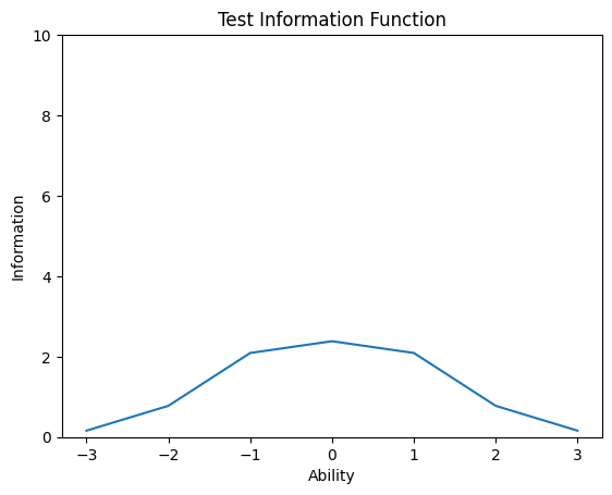

 

6.6 Interpreting the Test Informatin Function

어떤 부분은 솓아있고 어떤 부분은 낮아진다.

이를 해석하기 위해 분산을 사용한다

 

$$\text{SE}(\theta )=\frac{1}{\sqrt{I(\theta )}}$$

이는 2.283이 나오는데, 68%정도를 가리킨다.

 

 

6.7 Computer Session

6.7.1 Procedures for an Example Case

b=[-0.4,-0.3,-0.2,-0.1,0.0,0.0,0.1,0.2,0.3,0.4]
a=[1.0,1.5,1.2,1.3,1.0,1.6,1.6,1.4,1.1,1.7]
theta=np.arange(-3,3.1,0.1)
J=len(b)
ii=np.zeros((len(theta),J))
i=np.repeat(0,len(theta))
for j in range(J):
  P=1/(1+np.exp(-a[j]*(theta-b[j])))
  ii[:,j]=a[j]**2*P*(1.0-P)
  i=i+ii[:,j]

plt.plot(theta,i)
plt.xlabel('Ability')
plt.ylabel('Information')
plt.title('Test Information Function')
plt.yticks([0,2,4,6,8,10])
plt.show()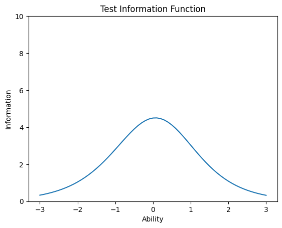

 

함수화

def tif(b,a=np.repeat(1,len(b)),c=np.repeat(0,len(b))):
  theta=np.arange(-3,3.1,0.1)
  J=len(b)
  ii=np.zeros((len(theta),J))
  i=np.repeat(0,len(theta))
  for j in range(J):
    Pstar=1/(1+np.exp(-a[j]*(theta-b[j])))
    P=c[j]+ (1-c[j])*Pstar
    ii[:,j]=a[j]**2*P*(1.0-P)**(Pstar/P)**2
    i=i+ii[:,j]

  plt.plot(theta,i)
  plt.xlabel('Ability')
  plt.ylabel('Information')
  plt.title('Test Information Function')
  plt.yticks([0,2,4,6,8,10])